This week we looked at how to determine if what you think you’re seeing in your data is actually there. It was a warp speed introduction to a big chunk of what humanity now knows about truth-finding methods. Most of the ideas behind the methods are centuries or sometimes millennia old, but they were very much fleshed out in the 20th century, and these profound ideas haven’t percolated through to all disciplines yet.

Slides.

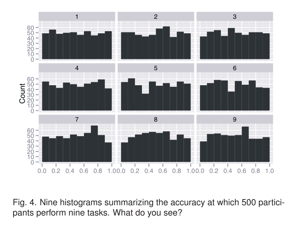
 “Figuring out what is true from what we can see” is called inference, and begins with a strong feel for how probability works, and what randomness looks like. Take a look at this picture (from the paper Graphical Inference for Infovis), which shows how well 500 students did on each of nine questions, each of which is scored from 0-100% correct.

Is there a pattern here? It looks like the answers on question 7 cluster around 75% and then drop off sharply, while the answers for question 6 show a bimodal distribution — students either got it or they didn’t.

Except that this is actually completely random synthetic data, drawn from a uniform distribution (equal chance of every score.) It’s very easy to make up narratives and see patterns that aren’t there — a human tendency called apohenia. To avoid fooling yourself, the first step is to get a feel for what randomness actually looks like. It tends to have a lot more structure, purely by chance, than most people imagine.

Here’s a real world example from the same paper. Suppose you’re interested to know if the pollution from the Texas oil industry causes cancer. Your hypothesis is that if refineries or drilling release carcinogens, you’ll see higher cancer rates around specific areas. Here’s a plot of the cancer rates for each county (darker is more cancer.) One of these plots is real data, the rest are randomly generated by switching the counties around. (click for larger.)

Can you tell which one is the real data? If you can’t tell the real data from the random data, well then, you don’t have any evidence that there is a pattern to the cancer rates.

In fact, if you show these pictures to people (look at the big version), they will stare at them for a minute or two, and then most folks will pick out plot #3 as the real data, and it is. This is evidence (but not proof) that there is a pattern there that isn’t random — because it looked different enough from the random patterns that you could tell which plot was real.

This is an example of a statistical test. Such tests are more typically done by calculating the odds that what you see has happened by chance, but this is a purely visual way to accomplish the same thing (and you can use this technique yourself on your own visualizations; see the the paper for the details.)

It’s part of the job of the journalist to understand the odds. In 1976, there was a huge flu vaccination program in the U.S. In early October, 14 elderly people died shortly after receiving the vaccine, three of them in one day. The New York Times wrote in an editorial,

It is conceivable that the 14 elderly people who are reported to have died soon after receiving the vaccination died of other causes. Government officials in charge of the program claim that it is all a coincidence, and point out that old people drop dead every day. The American people have even become familiar with a new statistic: Among every 100,000 people 65 to 75 years old, there will be nine or ten deaths in every 24-­‐hour period under most normal circumstances.

Even using the official statistic, it is disconcerting that three elderly people in one clinic in Pittsburgh, all vaccinated within the same hour, should die within a few hours thereafter. This tragedy could occur by chance, but the fact remains that it is extremely improbable that such a group of deaths should take place in such a peculiar cluster by pure coincidence.

Except that it’s not actually extremely improbable. Nate Silver addresses this issue in his book by explicitly calculating the odds:

Assuming that about 40 percent of elderly Americans were vaccinated within the first 11 days of the program, then about 9 million people aged 65 and older would have received the vaccine in early October 1976. Assuming that there were 5,000 clinics nationwide, this would have been 164 vaccinations per clinic per day. A person aged 65 or older has about a 1-­‐in-­‐7,000 chance of dying on any particular day; the odds of at least three such people dying on the same day from among a group of 164 patients are indeed very long, about 480,000 to one against. However, under our assumptions, there were 55,000 opportunities for this “extremely improbable” event to occur— 5,000 clinics, multiplied by 11 days. The odds of this coincidence occurring somewhere in America, therefore, were much shorter —only about 8 to 1

Silver is pointing out that the editorial falls prey to what might be called the “lottery fallacy.” It’s vanishingly unlikely that any particular person will win the lottery next week. But it’s nearly certain that someone will win. If there are very many opportunities for a coincidence to happen, and you don’t care which coincidence happens, then you’re going to see a lot of coincidences. You can see this effect numerically with even the rough estimation of the odds that Silver has done here.

Another place where probabilities are often misunderstood is polling. During the election I saw a report that Romney had pulled ahead of Obama in Florida, 49% to 47% with a 5.5% margin of error. I argued at the time that this wasn’t actually a story, because it was just too likely that Obama was actually still leading and the error in the poll was just that, error. In class we worked the numbers on this example and concluded that there was a 36% chance — so, 1 in 3 odds — that Obama was actually ahead (full writeup here.)

In fact, 5.5% is an unusually high error for a poll, so this particular poll was less informative than many. But until you actually run the numbers on poll errors a few times, you may not have a gut feel for when a poll result is definitive and when it’s very likely to be just noise. As a rough guide, a difference between two numbers of twice the margin of error is almost certain to indicate that the lead is real.

If you’re a journalist writing about the likelihood or unlikelihood of some event, I would argue that it is your job to get a numerical handle on the actual odds. It’s simply too easy to deceive yourself (and others!)

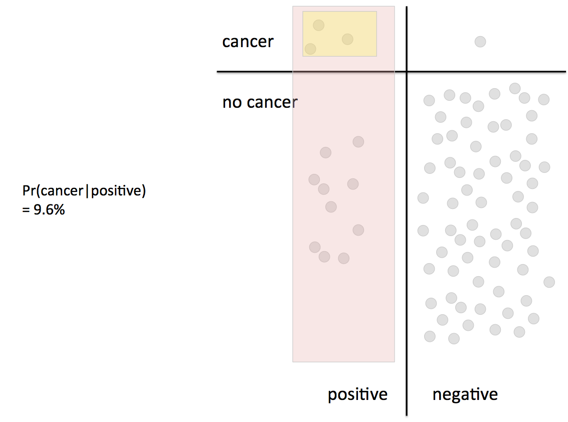
Next we looked at conditional probability — the probability that something happens given that something else has already happened. Conditional probabilities are important because they can be used to connect causally related events, but humans aren’t very good at thinking about them intuitively. The classic example of this is the very common base rate fallacy. It can lead you to vastly over-estimate the likelihood that someone has cancer when a mammogram is positive, or that they’re a terrorist if they appear on a watch list.

The correct way to handle conditional probabilities is with Bayes’ Theorem, which is easy to derive from the basic laws of probability. Perhaps the real value of Bayes’ theorem for this kind of problem is that it forces you to remember all of the information you need to come up with the correct answer. For example, if you’re trying to figure out P(cancer | positive mammogram) you really must first know the base rate of cancer in the general population, P(cancer). In this case it is very low because the example is about women under 50, where breast cancer is quite rare to begin with — but if you don’t know that you won’t realize that the small chance of false positives combined with the huge number of people who don’t have cancer will swamp the true positives with false positives.

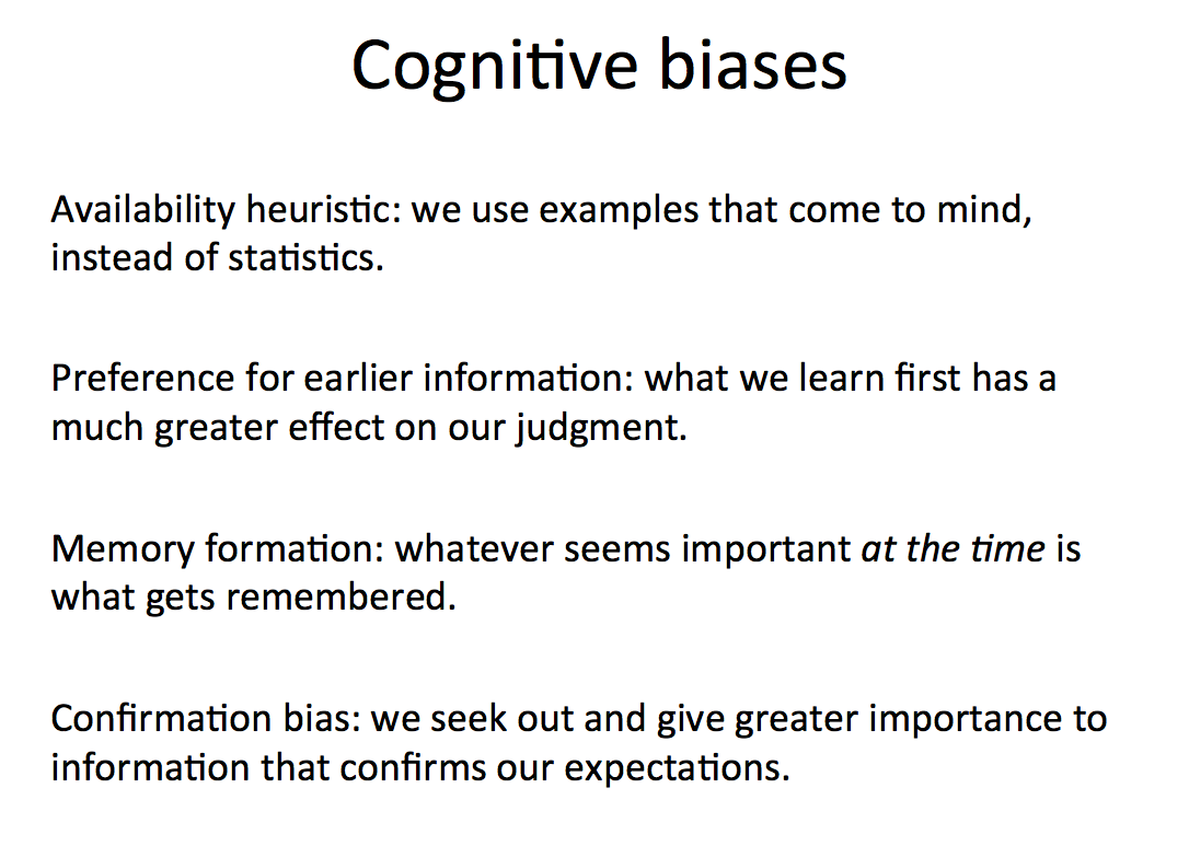
Then we switched gears from all of this statistical math and talked about how humans come to conclusions. The answer is, badly if you’re not paying attention. You can’t just review all the information you have on a story, think about it carefully, and come to the right conclusion. Our minds are simply not built this way. Starting in the 1970s an amazing series of cognitive psychology experiments revealed a set of standard human cognitive biases, unconscious errors that most people make in reasoning. There are lots of these that are applicable journalism.

The issue here is not that the journalist isn’t impartial, or acting fairly, or trying in good faith to get to the truth. Those are potential problems too, but this is a different issue: our minds don’t work perfectly, and in fact they fall short in predictable ways. While it’s true that people will see what they want to see, confirmation bias is mostly something else: you will see what you expect to see.

The fullest discussion of these startling cognitive biases — and also, conversely, how often our intuitive machinery works beautifully — is the book by one of the original researchers, Daniel Kahneman’s Thinking Fast and Slow. I also know of one paper which talks about how cognitive biases apply to journalism.

So how does an honest journalist deal with these? We looked at the method of competing hypotheses, as described by Heuer. The core idea is ancient, and a core principle of science too, but it bears repetition in modern terms. Instead of coming up with a hypothesis (“maybe there is a cluster of cancer cases due to the oil refinery”) and going looking for information that confirms it, come up with lots of hypothesis, as many as you can think of that explain what you’ve seen so far. Typically, one of these will be “what we’re seeing happened by chance,” often known as the null hypothesis. But there might be many others, such as “this cluster of cancer is due to more ultraviolet radiation at the higher altitude in this part of the country” or many other things. It’s important to be creative in the hypothesis generation step: if you can’t imagine it, you can’t discover that it’s the truth.

Then, you need to go look for discriminating evidence. Don’t go looking for evidence that confirms a particular hypothesis, because that’s not very useful; with the massive amount of information in the world, plus sheer randomness, you can probably always find some data or information to confirm any hypothesis. Instead you want to figure out what sort of information would tell you that one hypothesis is more likely than another. Information that straight out contradicts a hypothesis (falsifies it) is great, but anything that supports one hypothesis more than the others is helpful.

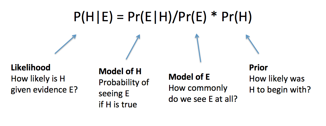
This method of comparing the evidence for different hypothesis has a quantitative equivalent. It’s Bayes’ theorem again, but interpreted a little differently. This time the formula expresses a relationship between your confidence or degree of belief in a hypothesis, P(H), the likelihood of seeing any particular evidence if the hypothesis is true, P(E|H), and the likelihood of seeing any particular piece of evidence whether or not the hypothesis is true, P(E)

To take a concrete example, suppose the hypothesis H is that Alice has a cold, and the evidence E is that you saw her coughing today. But of course that’s not conclusive, so we want to know the probability that she really does have a cold (and isn’t coughing for some other reason.) Bayes’ theorem tells us what we need to compute P(H|E) or rather P(cold|coughing)

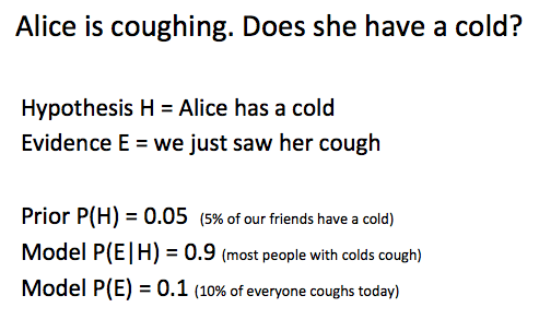
Under these assumptions, P(H|E) = P(E|H)P(H)/P(E) = 0.9 * 0.05 / 0.1 = 0.45, so there’s a 45% chance she has a cold. If you believe your initial estimates of all the probabilities here, then you should believe that there’s a 45% chance she has a cold.

But these are rough numbers. If we start with different estimates we get different answers. If we believe that only 2% of our friends have a cold at any moment then P(H) = 0.02 and P(H|E) = 18%. There is no magic to Bayesian inference; it can seem very precise but it all depends on the accuracy of your models, your picture of how the world works. In fact, examining the fit between models and reality is one of the main goals of modern statistics.

There’s probably no need to apply Bayes’ theorem explicitly to every hypothesis you have about your story. Heuer gives a much simpler table-based method that just lists supporting and disproving evidence for each hypothesis. Really the point is just to make you think comparatively about multiple hypothesis, and consider more scenarios and more discriminating evidence than you would otherwise. And not be so excited about confirmatory evidence.

However, there are situations where your hypotheses and data are sufficiently quantitative that Bayesian inference can be applied directly — such as election prediction. Here’s a primer on quantitative bayesian inference between multiple hypotheses. A vast chunk of modern statistics — most of it? — is built on top of Bayes’ theorem, so this is powerful stuff.

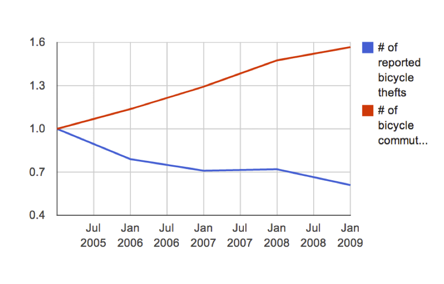
Our final topic was causality. What does it even mean to say that A causes B? This question is deeper than it seems, and a precise definition becomes critical when we’re doing inference from data. Often the problem that we face is that we see a pattern, a relationship between two things — say, dropping out of school and making less money in your life — and we want to know if one causes the other. Such relationships are called correlations, and probably everyone has heard by now that correlation is not causation.

In fact if we see a correlation between two different variables X and Y there are only a few real possibilities. Either X causes Y, or Y causes X, or Z causes both X and Y, or it’s just random fluke.

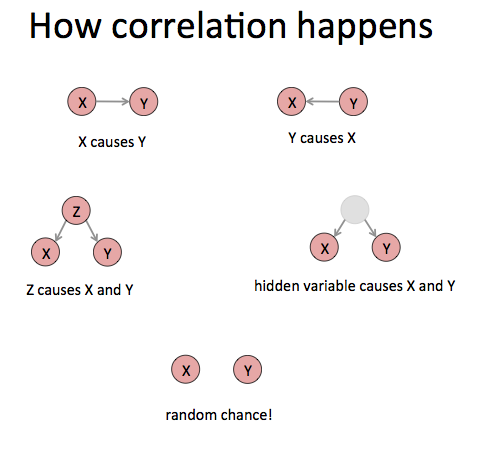
Our job as journalists is to figure out which one of these cases we are seeing. You might consider them alternate hypotheses that we have to differentiate between.

But if you’re serious about determining causation, what you actually want is an experiment: change X and see if Y changes. If changing X changes Y then we can definitely say that X causes Y (though of course it may not be the only cause, and Y could cause X too!) This is the formal definition of causation as embodied in the causal calculus. In certain rare cases you can prove cause without doing an experiment, and the causal calculus tells you when you can get away with this.

Finally, we discussed a real world example. Consider the NYPD stop and frisk data, which gives the date and location of each of the 600,000 stops that officers make on the street every year. You can plot these on a map. Let’s say that we get a list of mosque addresses, and discover that we discover that there are 15% more stops than average within 100 meters of New York City’s mosques. Given the NYPD history of spying on muslims, do we conclude that the police are targeting mosque-goers?

Let’s call that H1. How many other hypothesis can you imagine that will also explain this fact? (We came up with eight in class.) What kind of information or data or tests would you need to do to decide which hypothesis is the strongest?

The readings for this week were:

• The Psychology of Intelligence Analysis, chapters 1,2,3 and 8. Richards J. Heuer
• Correlation and causation, Business Insider
• If correlation doesn’t imply causation, then what does?, Michael Nielsen
• Graphical Inference for Infovis, Hadley Wickham et al.
• Why most published research findings are false, John P. A. Ioannidis

This week is about the analysis of networks of people, not the analysis of data on social networks. We might mine tweets, but fundamentally we are interested here in the people and their connections — the social network — not the content.

Slides.

Social networks have of course existed for as long as there have been people, and have been the subject of careful study since the early 20th century (see for example this 1951 study which compared groups performing the same a task using different network shapes, showing that “centrality” was an important predictor of behavior.) Recently it has become a lot easier to study social networks because of the amount of data that we all produce online — not just our social networking posts, but all of our emails, purchases, location data, instant messages, etc.

Different fields have different reasons to study social networks. In intelligence and law enforcement, the goal may be to identify terrorists or criminals. Marketing and PR  are interested in how people influence one another to buy things or believe things. In journalism, social network analysis is potentially useful in all four places where CS might apply to journalism. That is, social network analysis could be useful for:

• reporting, by identifying key people or groups in a story
• presentation, to show the user how the people in a story relate to one another
• filtering, to allow the publisher to target specific stories to specific communities
• tracking effects, by watching how information spreads

Because we’re going to have a whole week on tracking effects (see syllabus) we did not talk about that in class.

In a complex investigative story, we might use social network analysis to identify individual people or groups, based on who they are connected. This is what ICIJ did in their Skin and Bone series on the international human tissue trade. To present a complex story we might just simply show the social network of the people and organizations involved, as in the Wall Street Journal’s Galleon’s Web interactive on the famous insider trading scandal. I haven’t yet heard of anyone in journalism targeting specific audiences identified by social network analysis, but I bet it will happen soon.

Although visualization remains the main technique, there have been a number of algorithms designed for social network analysis. First there are multiple “centrality” measures, which try to determine who is “important” or “influential” or “powerful.” There are many of these.

But they don’t necessarily compute what a journalist wants to know. First, each algorithm is based on a specific assumption about how “things” flow through the network. Betweenness centrality assumes flows are always along the shortest path. Eigenvector centrality assumes a random walk. Whether this models the right thing depends on what is flowing — is it emails? information? money? orders? — and how you expect it to flow. Borgatti explains the assumptions behind centrality measures in great detail.

Often journalists are interested in “power” or “influence.” Unfortunately this is a very complicated concept, and while there is almost certainly some correlation between power and network centrality, it’s just not that simple. Communication Intermediaries — say, a secretary — may have extremely high betweeness centrality without any real authority.

Even worse, your network just may not contain the data you are actually interested in. You can produce a network showing corporate ownership, but if company A owns a big part of company B it doesn’t necessarily mean that A “controls” B. It depends on the precise relationship between the two companies, and how much autonomy B is given. Similar arguments can be made for links like “sits on the board of.”

This also brings up the point that there may be more than one kind of connection between people (or entities, more generally) in which case “social network analysis” is more correctly called “link analysis,” and if you use any sort of algorithm on the network you’ll have to figure out how to treat different types of links.

There are also algorithms for trying to find “communities” in networks. This requires a mathematical definition of a “cluster” of people, and one of the most common is modularity, which counts how many more intra-group edges there are than would be expected by chance in a graph with the same number of edges randomly placed.

Overall, social network analysis algorithms are useful in journalism, but not definitive. They are just not capable of understanding the complex context of a real-world social network. But the combination of a journalist and a good analysis system can be very powerful.

The readings were:

• Identifying the Community Power Structure, an old handbook for community development workers about figuring out who is influential by very manual processes. I hope this helps you think about what “power” is, which is not a simple topic, and traditional “analog” methods of determining it.
• Analyzing the data behind Skin and Bone, ICIJ. The best use of social network analysis in journalism that I am aware of.
• Sections I and II of Community Detection in Graphs. An introduction to a basic type of social network algorithm.
• Visualizing Communities, about the different ways to define a community
• Centrality and Network Flow, or, one good reason to be suspicious of centrality measures
• The Network of Global Corporate Control, a remarkable application of network analysis
• The Dynamics of Protest Recruitment Through an Online Network, good analysis of Twitter data from Spain “May 20” protest movement
• Exploring Enron, social network analysis of Enron emails, by Jeffrey Heer who went on to help create the D3 library

Here are a few other examples of the use of social network analysis in journalism:

• Visualizing the Split on Toronto City Council, a social network analysis that shows evolution over time
• Muckety, an entire site that only does stories based on link analysis
• Theyrule.net, an old map of U.S. boards of directors
• Who Runs Hong Kong?, a story explained through a social network analysis tool, South China Morning Post

Journalism has, historically, considered itself to be about text or other unstructured content such as images, audio, and video. This week we ask the questions: how much of journalism might actually be data? How would we represent this data? Can we get structured data from unstructured data?

Slides.

We start with Holovaty’s 2006 classic, A fundamental way newspaper sites need to change, which lays out the argument that the product of journalism is data, not necessarily stories. Central to this is the idea that it may not be humans consuming this data, but software that combines information for us in useful ways — like Google’s Knowledge Graph.

But to publish this kind of data, we need a standard to encode it. This gets us into the question of “what is a general way to encode human knowledge?” which has been asked by the AI community for at least 50 years. That’s why the title of this lecture is “knowledge representation.”

This is a hard problem, but let’s start with an easier one which has been solved: story metadata. Even without encoding the “guts” of a story as data, there is lots of useful data “attached” to a story that we don’t usually think about.

These details are important to any search engine or program that is trying to scrape the page. They might also include information on what the story is “about,” such as subject classification or a list of the entities (people, places, organizations) mentioned. There is a recent standard for encoding all of this sort of information directly within the page HTML, defined by schema.org which is a joint project of Google, Bing, and Yahoo. Take a look at the schema.org definition of a news article, and what it looks like in HTML. If you view the source of a New York Times, CNN, or Guardian article you will see these tags in use today.

In fact, every big news organization has its own internal schema, though some use it a lot more than others. The New York Times has been adding subject metadata since the early 20th century, as part of their (initially manual) indexing service. But we’d really like to be able to combine this type of information from multiple sources. This is the idea behind “linked open data” which is now W3C standard. Here’s Tim Berners-Lee describing the idea.

The linked data standard says each “fact” is described as a triple, in “subject relation object” form. Each of these three items is in turn either a literal constant, or a URL. Linked data is linked because it’s easy to refer to someone else’s objects by their URL. A single triple is equivalent to the proposition relation(subject,object) in mathematical logic. A database of triples is also called a “triplestore.”

There are many sites that already support this type of data. The W3C standard for expressing triples is an XML-based format called RDF, but there is also a much simpler JSON encoding of linked data. Here is what the “linked data cloud” looked like in 2010; it’s much bigger now and no one has mapped it recently.

The arrows indicate that one database references objects in the other. You will notice something called DBPedia at the center of the cloud. This is data derived from all those “infoboxes” on the right side of Wikipedia articles, and it has become the de-facto common language for many kinds of linked data.

Not only can one publisher refer to the objects of another publisher, but the standardized owl:sameAs relation can be used to equate one publisher’s object to a DBPedia object, or anyone else’s object. This expression of equivalence is an important mechanism that allows interoperability between different publishers. (As I mentioned above, every relation is actually a URL, so owl:sameAs is more fully known as http://www.w3.org/2002/07/owl#sameAs, but the syntax of many linked data formats allow abbreviations in many cases.)

DBPedia is vast and contains entries on many objects. If you go to http://dbpedia.org/page/Columbia_University_Graduate_School_of_Journalism you will see everything that DBPedia knows about Columbia Journalism School, represented as triples (the subject of every triple on this page is the school, so it’s implicit here.) If you go to http://dbpedia.org/data/Columbia_University_Graduate_School_of_Journalism.json you will get the same information in machine-readable format. Another important database is GeoNames, which contains machine readable information on millions of geographical entities worldwide — not just their coordinates but their shapes, containment (Paris is in France), and adjacencies. The New York Times also publishes a subset of their ontology as linked open data, including owl:sameAs relations that map their entities to DBPedia entities (example).

So what can we actually do with all of this? In theory, we can combine propositions from multiple publishers to do inference. So if database A says Alice is Bob’s brother, and database B says Alice is Mary’s mother, then we can infer that Bob is Mary’s uncle. Except that — as decades of AI research has shown — propositional inference is brittle. It’s terrible at common sense, exceptions, etc.

Perhaps the most interesting real-world application of knowledge representation is general question answering. Much like typing a question into a search engine, we allow the user to ask questions in human language and expect the computer to give us the right answer. The state of the art in this area is the DeepQA system from IBM, which competed and won on Jeopardy. Their system uses a hybrid approach, with several hundred different types of statistical and propositional based reasoning modules, and terabytes of knowledge both in unstructured and structured form. The right module is selected at run time based on a machine learning model that tries to predict what approach will give the correct answer for any given question. DeepQA uses massive triplestores of information, but they only contain a proposition giving the answer for about 3% of all questions. This doesn’t mean that linked data and its propositional knowledge is useless, just that it’s not going to be the basis of “general artificial intelligence” software. In fact linked data is already in wide use, but in specialized applications.

Finally, we looked at the problem of extracting propositions from text. The Reverb algorithm (in your readings) gives a taste of the challenges involved here, and you can search their database of facts extracted from 500 million web pages. A big part of proposition extraction is named entity recognition (NER). The best open implementation is probably the Stanford NER library, but the Reuters OpenCalais service performs a lot better, and you will use if for assignment 3. Google has pushed the state of the art in both NER and proposition extraction as part of their Knowledge Graph which extracts structured information from the entire web.

Your readings were:

• A fundamental way newspaper websites need to change, Adrian Holovaty
• The next web of open, linked data – Tim Berners-Lee TED talk
• Identifying Relations for Open Information Extraction, Fader, Soderland, and Etzioni (Reverb algorithm)
• Standards-based journalism in a semantic economy, Xark
• What the semantic web can represent – Tim Berners-Lee
• Building Watson: an overview of the DeepQA project
• Can an algorithm write a better story than a reporter? Wired/ 2012.

 

 

Sadly, we had to cut this lecture short because of Hurricane Sandy, but I’m posting the slides and a few notes.

You have no doubt seen lots of visualizations recently, and probably even studied them in your other classes (such as Data Journalism.) I want to give you a bit of a different perspective here, coming more from the information visualization (“infovis”) tradition which goes back to the beginnings of computer graphics in the 1970s. That culture recognized very early the importance of studying the human perceptual system, that is, how our eyes and brains actually process visual information.

Take a look at the following image.

You saw the red line instantly, didn’t you? Importantly, you didn’t have to think about this, or go look at each line, one at a time to find it, you “just saw it.” That’s because your visual cortex can do many different types of pattern recognition at a pre-conscious level. It doesn’t take any time or feel like any effort for you. This particular effect is called “visual pop-out” and many different types of visual cues can cause it.

The human visual system can also do pre-conscious comparisons of things like length, angle, size and color. Again, you don’t have to think about it know which line is longer.

In fact, your eye and brain are sensitive to dozens of visual variables simultaneously. You can think of these as “channels” which can be used to encode quantitative information. But not all channels are equally good for all types of information. Position and size are the most sensitive channels for continuous variables, while color and texture aren’t great for continuous variables but work well for categorical variables. The following chart, from Munzer, is a summary of decades of perceptual experiments.

This consideration of what the human visual system is good at — and there’s lot’s more — leads to what I call the fundamental principle of visualization: turn something you want to find into something you can see without thinking about. 

What kinds of “things” can we see in a visualization? That’s the art of visualization design! We’re trying to plot the data such that the features we are interested in are obviously visible. But here are some common data features that we can visualize.

The rest of the lecture — which we were not able to cover — gets into designing visualizations for big data. The key principle is, don’t try to show everything at once. You can’t anyway. Instead, use interactivity to allow the user to explore different aspects of the data. In this I am following the sage advice of Ben Fry’s Computational Information Design approach, and also drawing parallels to how human perception works. After all, we don’t “see” the entire environment at once, because only the central 2 degrees of our retina are sharp (the fovea.) Instead we move our eyes rapidly to survey our environment. Scanning through big data should be like this, because we’re already built to understand the world that way.

In the final part of the lecture — which we actually did cover, briefly — we discussed narrative, rhetoric and interpretation of visualizations. Different visualizations of the same data can “say” completely different things. We looked at a simple line graph and asked, what are all the editorial choices that went into creating it?

I can see a half dozen choices here; there are probably more.

• The normalization used — all values are adjusted relative to Jan 2005 values
• Choice of line chart (instead of any other kind)
• Choice of color. Should thefts be blue, or would red have been better?
• Time range. The data probably go back farther.
• Legend design.
• Choice of these data at all, as opposed to any other way to understand bicycle use and thefts.

Also, no completed visualization is entirely about the data. If you look at the best visualization work, you will see there there are “layers” to it. These include:

• The data. What data is chosen, what is omitted, what are the sources.
• Visual representation. How is the data turned into a picture.
• Annotation. Highlighting, text explanations, notes, legends.
• Interactivity. Order of presentation, what the user can alter.

In short, visualization is not simply a technical process of turning data into a picture. There are many narrative and editorial choices, and the result will be interpreted by the human perceptual system. The name of the game is getting a particular impression into the user’s head, and to do that, you have to a) choose what you want to say and b) understand the communication and perception processes at work.

Readings for this week were:

• Visual Encoding, Michael Dubakov
• Computational Information Design chapters 1 and 2, Ben Fry
• Journalism in an age of data, Geoff McGhee (an hour long documentary!)
• Visualization Rhetoric: Framing Effects in Narrative Visualization, Hullman and Diakopolous
• Visualization, Tamara Munzner

I also recommend the book Designing Data Visualizations.

For this assignment you will evaluate the performance of OpenCalais, a commercial entity extraction service. You’ll do this by building a text enrichment program, which takes plain text and outputs HTML with links to the detected entities. Then you will take five random articles from your data set, enrich them, and manually count how many entities OpenCalais missed or got wrong.

1. Get an OpenCalais API key, from this page.

2. Install the python-calais module. This will allow you to call OpenCalais from Python easily. First, download the latest version of python-calais. To install it, you just need calais.py in your working directory. You will probably also need to install the simplejson Python module. Download it, then run “python setup.py install.” You may need to execute this as super-user.

3. Call OpenCalais from Python. Make sure you can successfully submit text and get the results back, following these steps. The output you want to look at is in the entities array, which would be accessed as “results.entities” using the variable names in the sample code. In particular you want the list of occurrences for each entity, in the “instances” field.

>>> result.entities[0]['instances']
[{u'suffix': u' is the new President of the United States', u'prefix': u'of the United States of America until 2009.  ', u'detection': u'[of the United States of America until 2009.  ]Barack Obama[ is the new President of the United States]', u'length': 12, u'offset': 75, u'exact': u'Barack Obama'}]
>>> result.entities[0]['instances'][0]['offset']
75
>>>

Each instance has “offset” and “length” fields that indicate where in the input text the entity was referenced. You can use these to determine where to place links in the output HTML.

4. Read from stdin, create hyperlinks, write to stdout. Your Python program should read text from stdin and write HTML with links on all detected entities to stdout. There are two cases to handle, depending on how much information OpenCalais gives back.

In many cases, like the example in the previous step, OpenCalais will not be able to give you any information other than the string corresponding to the entity, result.entities[x][‘name’]. In this case you should construct a Wikipedia link by simply appending to the name to a Wikipedia URL, converting spaces to underscores, e.g.

http://en.wikipedia.org/wiki/Barack_Obama

In other cases, especially companies and places, OpenCalias will supply a link to an RDF document that contains more information about the entity. For example.

>>> result.entities[0]{u'_typeReference': u'http://s.opencalais.com/1/type/em/e/Company', u'_type': u'Company', u'name': u'Starbucks', '__reference': u'http://d.opencalais.com/comphash-1/6b2d9108-7924-3b86-bdba-7410d77d7a79', u'instances': [{u'suffix': u' in Paris.', u'prefix': u'of the United States now and likes to drink at ', u'detection': u'[of the United States now and likes to drink at ]Starbucks[ in Paris.]', u'length': 9, u'offset': 156, u'exact': u'Starbucks'}], u'relevance': 0.314, u'nationality': u'N/A', u'resolutions': [{u'name': u'Starbucks Corporation', u'symbol': u'SBUX.OQ', u'score': 1, u'shortname': u'Starbucks', u'ticker': u'SBUX', u'id': u'http://d.opencalais.com/er/company/ralg-tr1r/f8512d2d-f016-3ad0-8084-a405e59139b3'}]}
>>> result.entities[0]['resolutions'][0]['id']
u'http://d.opencalais.com/er/company/ralg-tr1r/f8512d2d-f016-3ad0-8084-a405e59139b3'
>>>

In this case the resolutions array will contain a hyperlink for each resolved entity, and this is where your link should go. The linked page will contain a series of triples (assertions) about the entity, which you can obtain in machine-readable from by changing the .html at the end of the link to .json. The sameAs: links are particularly important because they tell you that this entity is equivalent to others in dbPedia and elsewhere.

Here is more on OpenCalias’ entity disambiguation and use of linked data.

5. Pick five random documents and enrich them. Choose them from the document set you worked with in Assignment 1.  It’s important that you actually choose randomly — as in, use a random number generator. If you just pick the first five, there may be biases in the result. Using your code, turn each of them into an HTML doc.

6. Read the enriched documents and count to see how well OpenCalais did. You need to read each output document very carefully and count three things:

• Entity references. Count each time there is a name of a person, place, or organization, including pronouns (such as “he”) or other references (like “the president.”)
• Detected references. How many of these did OpenCalais find?
• Correct references. How many of the links go to the right page? Did our hyperlinking strategy (OpenCalais RDF pages where possible, Wikipedia when not) fail to correctly disambiguate any of the references, or, even worse, disambiguate any to the wrong object?

7. Turn in your work. Please turn in:

• Your code
• The enriched output from your documents
• A brief report describing your results.

The report should include a table of the three numbers — references, detected, correct — for each document, as well as overall percentages across all documents. Also report on any patterns in the failures that your see. Where is OpenCalais most accurate? Where is it least accurate? Are there predictable patterns to the errors?

Due before class on Monday, November 19.

 

For this assignment you will design a hybrid filtering algorithm. You will not implement it, but you will explain your design criteria and provide a filtering algorithm in sufficient technical detail to convince me that it might actually work — including psuedocode.

You may choose to filter:

• Facebook status updates, like the Facebook news feed
• Tweets, like Trending Topics or the many Tweet discovery tools
• The whole web, like Prismatic
• something else, but ask me first

Your filtering algorithm can draw on the content of the individual items, the user’s data, and other users’ data. The assignment goes like this:

1. List all available information that you have available during the debate. If you want to filter Facebook or Twitter, you may pretend that you are either of these companies and have access to all of their tweets etc. You also also assume you have a web crawler or a firehose of every RSS feed or whatever you like, but you must be specific and realistic about what data you are operating with.

2. Argue for the design factors that you would like to influence the filtering, in terms of what is desirable to the user, what is desirable to the publisher (e.g. Facebook or Prismatic), and what is desirable socially. Explain as concretely as possible how each of these (probably conflicting) might be achieved through in software. Since this is a hybrid filter, you can also design social software that asks the user for certain types of information (e.g. likes, votes, ratings) or encourages users to act in certain ways (e.g. following) that generate data for you.

3. Write psuedo-code for a function that produces a “top stories” list. This function will be called whenever the user loads your page or opens your app, so it must be fast and frequently updated. You can assume that there are background processes operating on your servers if you like. Your psuedo-code does not have to be executable, but it must be specific and unambiguous, such that a good programmer could actually go and implement it. You can assume that you have libraries for classic text analysis and machine learning algorithms.

4. Write up steps 1-3. The result should be no more than five pages. However, you must be specific and plausible. You must be clear about what you are trying to accomplish, what your algorithm is, and why you believe your algorithm meets your design goals (though of course it’s impossible to know for sure without testing; but I want something that looks good enough to be worth trying.)

The assignment is due before class on  Monday, October 29.

 

In previous weeks we discussed filters that are purely algorithmic (such as NewsBlaster) and filters that are purely social (such as Twitter.) This week we discussed how to create a filtering system that uses both social interactions and algorithmic components.

Slides.

Here are all the sources of information such an algorithm can draw on.

We looked at two concrete examples of hybrid filtering. First, the Reddit comment ranking algorithm, which takes the users’ upvotes and downvotes and sorts not just by the proporition of upvotes, but by how certain we are about proportion, given the number of people who have actually voted so far. Then we looked at item-based collaborative filtering, which is one of several classic techniques based on a matrix of users-item ratings. Such algorithms power everything from Amazon’s “users who bought A also bought B” to Netflix movie recommendations to Google News’ personalization system.

Evaluating the performance of such systems is a major challenge. We need some metric, but not all problems have an obvious way to measure whether we’re doing well. There are many options. Business goals — revenue, time on site, engagement — are generally much easier to measure than editorial goals.

Finally, we saw a presentation from Dr. Aria Haghighi, co-founder of the news personalization service Prismatic, on how his system crawls the web to find diverse articles that match user interests.

The readings for this week were:

• Item-Based Collaborative Filtering Recommendation Algorithms, Sarwar et. al
• How Reddit Ranking Algorithms Work, Amir Salihefendic
• Google News Personalization: Scalable Online Collaborative Filtering, Das et al
• Slashdot Moderation, Rob Malda
• Pay attention to what Nick Denton is doing with comments, Clay Shirky
• How does Google use human raters in web search?, Matt Cutts

This concludes our work on filtering systems — except for Assignment 2.

This is the first of three weeks on “filtering.” We define that word by looking at a feedback model of journalism: a journalist observes something happening in the world, produces a story about it, the user consumes the story, and then they potentially act in some way that changes the world (such as voting, choosing one product over another, protesting, or many other possible outcomes.) This follows David Bornstein’s comment that “journalism is a feedback mechanism to help society self-correct.”

This diagram is missing something obvious: there are lots and lots of topics in the world, hence many stories. Not every potential story is written, and not every written story is consumed by every user.

This is where “filtering” comes in, the arrow on the bottom right. Somehow, the user sees only a subset of all produced stories. The sheer, overwhelming logic of the amount of journalism produced versus hours in the day requires this (and we illustrated this with some numerical examples in the slides.)

(Incidentally, journalism as an industry has mostly been involved with story production, the upper-right arrow, and more recently has been very concerned about how fewer reporters result in more stories not covered, the upper left arrow. The profession has, historically, payed much less attention to the effects of its work, bottom left, and the filtering problem, bottom right.)

(There is another major thing missing from this diagram: users now often have access to the same sources as journalists, and in any case journalism is now deeply participatory. We’ll talk a lot more about this next week.)

This week we focussed on purely algorithmic filtering. As a concrete example, we examined the inner workings of the Columbia Newsblaster system, a predecessor of Google News which is conveniently well documented.

Slides for week 4.

The readings (from the syllabus) were mostly to get you thinking about the general problem of information overload and algorithmic filtering, but the Newsblaster paper is also in there.

• Who should see what when? Three design principles for personalized news Jonathan Stray
• Tracking and summarizing news on a daily basis with Columbia Newsblaster, McKeown et al
• Guess what? Automated news doesn’t quite work, Gabe Rivera
• The Hermeneutics of Screwing Around, or What You Do With a Million Books, Stephen Ramsay
• Can an algorithm be wrong?, Tarleton Gillespie
• The Netflix Prize, Wikipedia

Actually, much of the guts of Newsblaster is in this paper on their on-line clustering algorithm that groups together all stories which are about the same underlying event. Note the heavy reliance on our good friends from last week: TF-IDF and cosine distance. The graphs in this paper show that for this problem, you can do better than TF-IDF by adding features corresponding to extracted entities (people, places, dates) but really not by very much.

We wrapped up with a discussion about the problem of algorithmic filter design. We defined this problem on two levels. In terms of functional form,

and in terms of the much more abstract desirable attributes

 The great challenge is to connect these two levels of description: to express our design criteria in terms of an algorithm. Here are the notes from our brief discussion about how to do this.

On the right we have interest, effects, agency, my proposed three criteria for “when should a user see a story.” Somehow, these have to be expressed in terms of computational building blocks like TF-IDF and all of the various signals available to the algorithm.  That’s what the fuzzy arrow is… there’s a gap here, and it’s a huge gap.

On the left are some of the factors to consider in trying to assess whether a particular story is interesting, will effect, or can be acted on by a particular user: geo information (location of user and story), user’s industry and occupation, other user demographics, the people in the user’s social network, the “content” they’ve produced (everything they’ve ever tweeted, blogged, etc.), and the time or duration of the story event. We can also offload parts of the selection process to the user, by showing multiple stories or types of stories and having the user pick. Similarly we can offload parts of the problem to the story producer, who might use various techniques to try to target a particular story to a particular group of people. We’ll talk extensively about including humans in the filtering system in the next two weeks.

The bracket and 2^N notation just means that any combination of these factors might be relevant. E.g. location and occupation together might be a key criteria.

In the center of the board I recorded one important suggestion: we can use machine learning to teach the computer which are the right articles for each factor. For example, suppose we’re trying to have the algorithm decide which stories are about events that affect people in different occupations. For each occupation, a human can collect many stories that someone in that occupation would want to read, then we can take the average of the TF-IDF vectors of those stories to define a subject category. The computer can then compare each incoming story to the corresponding coordinate for each user’s occupation.

I don’t know whether this particular scheme will work, but having the humans teach the computers is an essential idea — and one that is very common in search engines and filtering systems of all kinds.

 

I’m altering the structure of the assignment a little bit from the version in the original syllabus, in the hopes of making it more interesting. We may even be able to learn and document somethings that seem to be missing from the literature.

The assignment goes like this:

1) Get your data into a standard format. You have all now chosen a dataset that contains, at least in part, a significant text corpus. Your first task will be to scrape, format, or otherwise coerce this information into a convenient format for Python to read.

I recommend a very simple format: plain text, one document per line, all documents in one file.

It’s not completely trivial to get the documents in this format, but it shouldn’t be hard either. The first task is to extract plain text from your documents. If your source material is PDF, you can use the pdftotext command (pre-installed on Macs, available for Windows and Linux as part of xpdf). If it’s HTML, you may want to delete matches to the regex /<[^>]*>/ to remove all tags; you may also want to scrape the content of a particular div, as opposed to the whole page source. If you need to scrape your data from web pages, I heartily recommend writing a little script within the ScraperWiki framework.

Obviously this one-document-per-line format can’t represent the newlines in the original document, but that’s ok, because we’re going to throw them out during tokenization anyway. So you can just replace them with spaces.

2) Feed the data into gensim. Now you need to load the documents into Python and feed them into the gensim package to generate tf-idf weighted document vectors. Check out the gensim example code here. You will need to go through the file twice: once to generate the dictionary (the code snippet starting with “collect statistics about all tokens”) and then again to convert each document to what gensim calls the bag-of-words representation, which is un-normalized term frequency (the code snippet starting with “class MyCorpus(object)”

Note that there is implicitly another step here, which is to tokenize the document text into individual word features — not as straightforward in practice as it seems at first, but the example code just does the simplest, stupidest thing, which is to lowercase the string and split on spaces. You may want to use a better stopword list, such as this one.

Once you have your Corpus object, tell gensim to generate tf-idf scores for you like so.

3) Do topic modeling. Now you can apply Latent Semantic Indexing or Latent Dirichlet Allocation to the tf-idf vectors, like so. You will have to supply the number of dimensions to keep. Figuring out a good number is part of the assignment. Note that you dont have to do topic modeling — this is really a dimensionality reduction / de-noising step, and depending on your documents and application, may not be needed. If you want to try working with the original tf-idf vectors, that’s OK too. That’s what Overview does.

4) Analyze the vector space. So now you have a bunch of vectors in a space of some dimension, each of which represents a document, and we hope that similar documents are close in this space (as measured by cosine distance.) Have we gotten anywhere? There are several things we could do at this point:

1. Choose particular document, then find the k closest documents. Are they related? How? (Read the text of the documents to find out) How big do you have to make k before you see documents that seem unrelated?
2. Run a clustering algorithm, such as any of those in the python cluster package. Then look at the documents in each cluster, again reading their text and reporting on the results. Non-hierarchical clustering algorithms generally take the number of clusters as a parameter, while with hierarchical clusterings you have a choice of what level of the tree to examine. How do these choices affect what you see?
3. Or, you could run multi-dimensional scaling to plot the entire space in 2D, perhaps with some other attribute (time? category?) as a color indicator variable. This is probably best done in R. To get your document vectors into R, write them out of gensim in the MatrixMarket format, then load them in R (remember you’ll need to do “library(Matrix)” first to make readMM available in R.) Then you’ll want to compute a distance matrix of the documents, run mdscale on it, and plot the result like we did in the House of Lords example.
4. If you did LSI or LDA topic modeling, what do the extracted topics look like? Do they make any sort of human sense? Can you see examples of polysemy or synonymy? If you pull out the k docs with the highest score on a particular topic, what do you find? How many documents have no clear primary topic? What do the low-order topics (far down the dimension list) look like? How many dimensions until it just seems like noise?

Your assignment is to do one of these things, whichever you think will be most interesting. You may also discover that it is hard to interpret the results without trying some of the other techniques. Actually, figuring out how, exactly, to evaluate the clustering is part of this assignment. Hint: one useful idea is to ask, how might a human reporter organize your documents? Where did the computer go wrong?

You will of course need to implement cosine distance either in Python or R to make any of these go. This should be only a few lines…

5) Compare to a different algorithmic choice. Now do steps 3 and 4 again, with a different choice of algorithm or parameter. The point of this assignment is to learn how different types of clustering give qualitatively different results on your document set… or not. So repeat the analysis, using either:

• a different topic modeling algorithm. If you used plain tf-idf before, try LSI or LDA. Or if you tried LSI, try LDA. Etc.
• a different number of clusters, or a different level in the hierarchical clustering tree.
• a different number of output dimensions to LSI or LDA.
• a different distance function
• etc.

I want to know which of your two cases gives “better” results. What does “better” mean? It depends very much on what the interesting questions are for your data set. Again, part of the assignment is coming up with criteria to evaluate these clusterings. Generally, more or easier insight is better. (If the computer isn’t making your reporting or filtering task significantly easier, why use it?)

6) Write up the whole thing. I will ask you to turn in your the code you wrote but that’s really only to confirm that you actually did all the steps. I am far more interested in what you have learned about the best way to use these algorithms on your data set. Or if you feel you’ve gained little or no insight into your data set using these techniques, explain why, and suggest other ways to explore it.

This assignment is due Monday, October 15 at 4:00 PM. You may email me the results. I am available for questions by email before then, or in person at office hours on Thursday afternoons 1-4.